The Cost of Variability

What Investors Miss When They Focus on System Targets Instead of Behavior

In humans, blood pH is tightly controlled between 7.35 and 7.45. Small deviations cause dysfunction. Larger ones are fatal. We understand this intuitively: the body does not tolerate instability.

Now consider how we evaluate aquaculture systems.

Investors are typically shown target conditions — temperature, oxygen, pH — presented as if they describe how the system operates. A model might state that the system runs at 12°C, with oxygen above 85% saturation, and pH at 7.0. These numbers look precise. They feel reassuring.

But they don’t describe the system.

They describe the intention.

System Behaviour

Biological systems are not defined by their targets. They are defined by how they behave over time.

A production model might assume “the system operates at pH 7.0,” but real systems don’t operate at a number. They operate across a range. And more importantly, they deviate. During feeding, biomass accumulation, sea lice treatments, handling, harvest, smolt transfer, and routine operational disturbances, conditions move away from target and then return — or attempt to.

These deviations are often described as temporary. Which is true, but also misleading. Because the economic impact is not driven by whether a deviation occurs. It is driven by how often the system leaves its optimal state, and how long it stays there.

The Cost of Compensation

Fish can tolerate a wider range of environmental pH than humans, but they do not do so passively. When conditions shift, they actively compensate through ion exchange at the gills, acid–base buffering, and changes in respiration. That capacity for compensation is what allows them to survive variability. But it is not free.

A single pH excursion during a treatment is rarely the problem. What matters is repetition. How often do these excursions occur? How quickly does the system recover? And does recovery complete before the next deviation begins?

High-intensity systems tend to generate variability continuously. Feeding cycles, CO₂ accumulation, biofilter dynamics, and density-dependent effects all contribute to a system that is not operating at steady state, but in a continuous cycle of deviation and correction. Over time, the system spends less time at its optimal condition and more time managing its own instability.

The Impact on Financial Performance

This rarely appears explicitly in financial models. But it shows up indirectly, in ways that are easy to miss and difficult to attribute. Growth slows. Appetite softens. Feed conversion drifts. Production cycles extend. Interventions increase. Size distributions widen. Individually, these effects are modest. Collectively, they define performance.

For investors, this creates a problem. Most production models are built around steady-state assumptions. They describe what the system should do under stable conditions. But real systems are not stable. They oscillate. And the economics are not driven by the average condition, but by the frequency, magnitude, and duration of deviations from optimal.

This suggests a different way to interrogate a production plan.

Challenging the Production Plan

Instead of starting with the target conditions, start with the variability. What range is considered optimal, and what range is acceptable? How much time does the system actually spend within those bounds? What operational events drive deviations, and how frequently do they occur? Are these events continuous, like feeding and biomass accumulation, or episodic, like treatments and transfers? And how long does it take for the system to recover — not in theory, but in practice, and especially at peak biomass?

This last point matters more than it appears. Many systems are stable early in the production cycle, when biomass is low and demand on the system is limited. The question is what happens as density increases. Does variability remain controlled, or does it expand? If stability degrades at peak biomass, the system’s practical capacity may be materially lower than its design capacity.

This is the core insight: most investment cases assume stability, but real systems behave differently. They move. And that movement has a cost.

How to Quantify These Costs

At some point, every investment discussion converges on valuation, and with it, the question of what discount rate to apply. In a Net Present Value framework, the discount rate is meant to reflect risk. When a system feels uncertain, the instinct is to increase the rate.

But this is where things often go wrong.

The risk embedded in high-intensity aquaculture systems is not abstract. It is operational. It does not primarily affect the time value of money. It affects the reliability of the cash flows themselves.

Variability expresses itself upstream of valuation, through lower effective growth rates, worse feed conversion, longer production cycles, reduced survival, higher operating costs, and ultimately, constrained throughput. These are not financial assumptions. They are biological realities. And they directly determine the cash flows being discounted.

A system might be designed to produce 10,000 tonnes per year. On paper, that capacity flows cleanly into revenue, margin, and valuation. But under real operating conditions, variability introduces friction. Growth slows. Recovery lags. Cycles extend. Constraints bind earlier than expected. And realized output becomes 8,000 to 8,500 tonnes.

That difference is not a rounding error. It is the cost of instability.

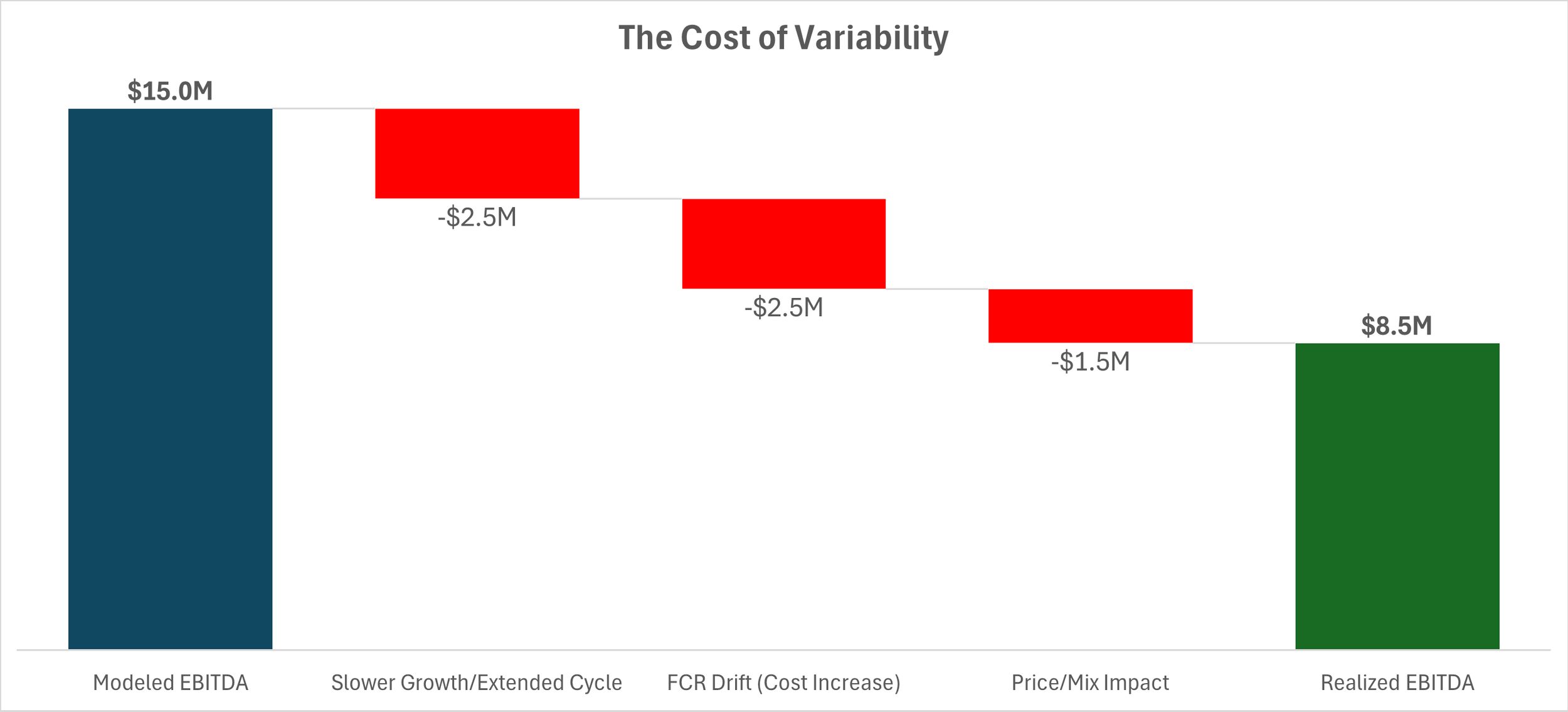
Impact of variability on system performance.

Embedded Discounting

You can think of this as a form of embedded discounting — not applied to the rate, but applied to the output. The system does not lose value because the discount rate is wrong. It loses value because it cannot consistently deliver what the model assumes.

Changing the discount rate by a few percentage points will move valuation. But getting the biology wrong changes the cash flows entirely. And in many cases, the gap between modeled and realized performance is far larger than any reasonable adjustment to the discount rate.

Fish can tolerate variability. But they do not do so for free. And in high-intensity systems, variability is not an exception. It is the operating condition.

For investors, the question is simple.

Is that variability understood, managed, and reflected in the model?

Or assumed away?