Why Some Aquaculture Projects Look Profitable — and Aren’t

Aquaculture projects are often evaluated using inconsistent frameworks. Land-based farms may be treated as infrastructure, offshore systems compared to shipping, and net-pen farms viewed as agriculture.

Each comparison carries implicit assumptions about risk, asset life and capital efficiency. The result is that projects with very similar economics can end up being evaluated through entirely different lenses.

This article proposes a simple framework for comparing them.

The Basic Financial Question

At its core, every investment decision comes down to a simple comparison:

Does the value created by the project exceed the capital required to build it?

In finance, that comparison is usually expressed through net present value (NPV).

NPV converts the future cash flows into today’s dollars and compares them with the initial investment. It’s basically the phrase “a bird in hand is worth two in the bush” translated to finance terms – money today is inherently worth more than money potentially earned in the future.

If the NPV is positive, the project creates value. If it is negative, the investment destroys value.

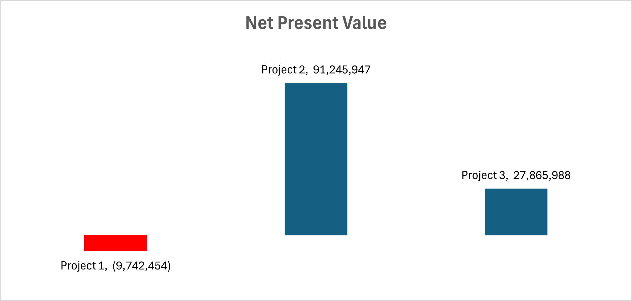
NPV Comparison

Discount Rates and Risk

The discount rate reflects the level of risk investors believe they are taking and the price (or cost of money) they assign to that risk. Higher-risk projects require higher discount rates because investors demand greater compensation for uncertainty.

Different types of assets tend to attract different discount rates.

Asset Type

Typical Discount Rate Range

Government bonds 2–4%

Regulated infrastructure (utilities, pipelines) 5–7%

Mature industrial businesses 7–10%

Commercial real estate 8–12%

Shipping / commodity assets 10–14%

Private equity investments 15–20%

Venture capital / early-stage technologies 20–30%+

This is one reason aquaculture projects can be difficult to compare. Investors often place them into different categories before the analysis even begins.

Residual Value

Most project models assume that an asset will continue to have some value at the end of the forecast period. Usually captured through a residual value assumption which represents the economic value of the asset at the end of the model horizon — whether because the facility can continue operating, be sold, or retains some salvage value. They can have a significant impact on valuation.

Aquaculture assets are difficult to value accurately. They operate continuously in highly corrosive environments and contain many mechanical systems. An overly optimistic residual value can significantly distort a project NPV.

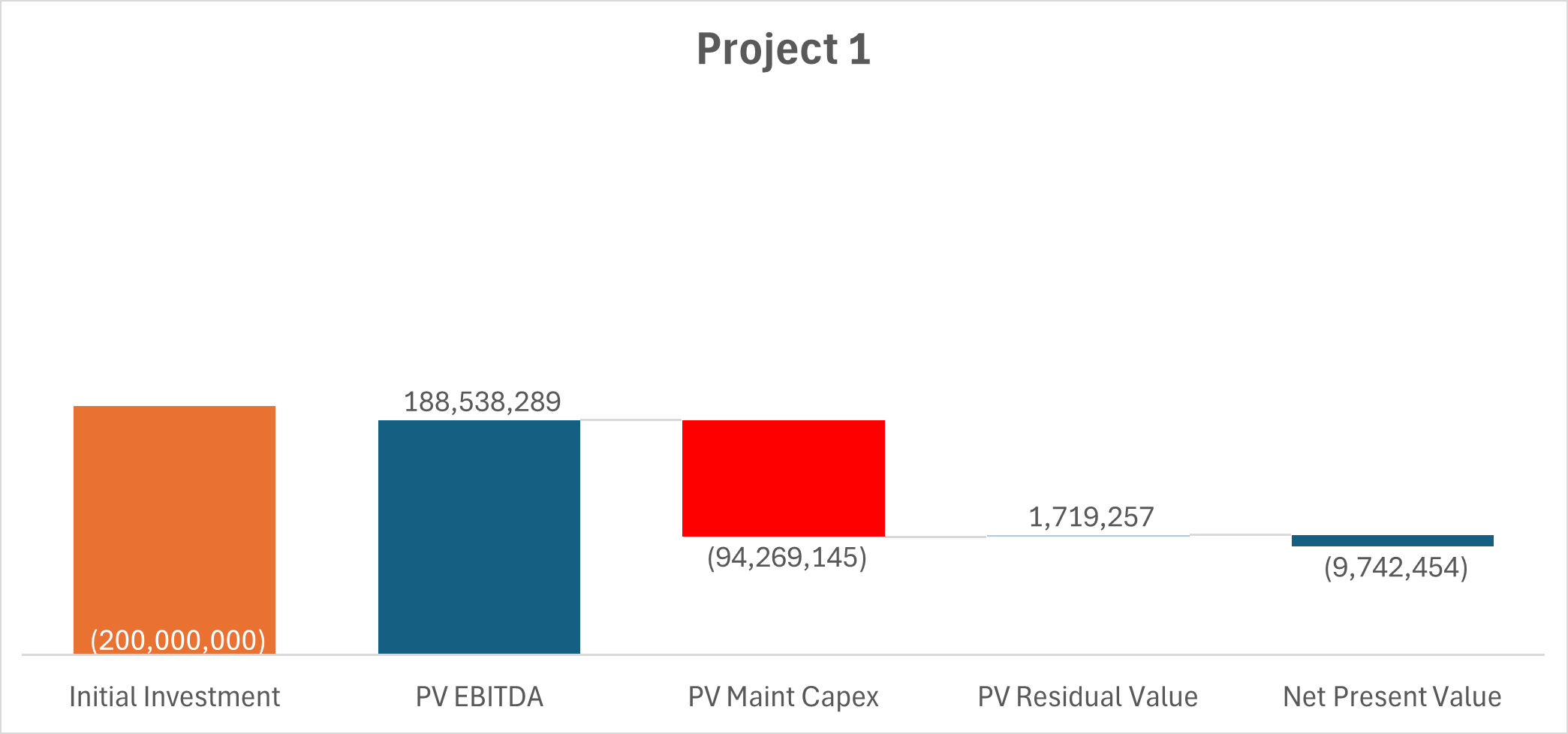
Breaking the Economics into Components

In simplified terms, project value can be thought of as the difference between the operating value generated by the system and the capital required to build and maintain it.

While the mechanics of NPV can look complex, the economics of most aquaculture projects can be broken down into a handful of components:

Initial Investment
The capital investment required to build the production system.

PV EBITDA
The present value of the operating earnings generated by the farm over the planned life of the project.

PV Maintenance Capex
The present value of the capital required to maintain the system over time.

PV Residual Value
The present value of the asset at the end of the modeled period.

Biological Performance
Project economics are built around key inputs and outputs – harvests, mortality, operating density.

Once these elements are separated, projects become much easier to compare.

Why This Matters

In discussions about aquaculture investments, attention often focuses on headline metrics such as projected production volumes or EBITDA per kilogram.

Those metrics are important, but they can also be misleading.

Two projects might theoretically generate similar operating earnings, but if one requires more capital to build or maintain, is more difficult or risky to operate or has an unrealistic assumption regarding residual value, the investment outcome can be dramatically different.

Biological Performance and Production Systems

A farm is assumed to produce a certain volume of fish each year, and the economics are built around that output.

During operations, growth rates, feed conversion efficiency, oxygen availability, fish health and survival are highly volatile. Small disruptions can lead to outsized financial consequences.

These effects are modelled through a set of biological performance factors:

• Working capacity – the proportion of theoretical capacity that can be utilized

• Survival rate – the share of stocked fish that reach harvest

• Harvest realization – the extent to which harvested fish achieve expected size and value.

These factors are combined to estimate effective output relative to design capacity.

A facility designed to produce 10,000 tonnes annually but operating at 80% of capacity carries the same capital investment while generating substantially less output.

In many infrastructure investments — pipelines, power plants or transportation assets — utilization rates tend to be relatively stable once the asset is built. Aquaculture systems, by contrast, must continually maintain biological stability to achieve their design performance. Maintaining system stability can become harder as systems age.

A Simple Comparison Tool

To illustrate this framework, I built a simple model that allows three aquaculture production scenarios to be compared using a small number of assumptions.

The model allows users to adjust:

• production capacity

• EBITDA per kilogram

• capital cost

• sustaining capital requirements

• asset life

• discount rate

• biological performance.

From these inputs, the model calculates the present value of operating earnings, maintenance capital and residual value, and compares them with the initial investment.

The results are presented through simple waterfall charts that show how each component contributes to the final investment outcome.

What the Model Reveals

When different scenarios are tested, an interesting pattern usually emerges.

Changes in assumptions about biological performance and maintenance capital often have a far larger impact on valuation than changes in discount rates or residual value assumptions.

In other words, the factors that ultimately determine whether an aquaculture investment succeeds or fails are usually operational rather than financial.

This is not surprising for those working inside the industry. Aquaculture systems are biological production environments, not purely financial assets.

But financial models do not always make that distinction clear.

The purpose of this framework is not to predict which production systems will succeed. It is simply to provide a clearer way of comparing the assumptions that ultimately determine whether an aquaculture investment creates or destroys value.

Download the Model

Readers can experiment with these assumptions using the simple model linked below.

Feedback and comments welcomed.